Searching Algorithms in AI ( Uninformed )

---

---

In AI, the universal technique for problem-solving is searching. For a given problem, it is needed to think of all possible ways to attain the existing goal state from its initial state. Searching in AI can be defined as a process of finding the solution for a given set of problems. A searching strategy is used to specify which path is to be selected to reach the solution.

Terminologies in Search Algorithms

• Search: A step-by-step procedure to solve a given search problem.  Three main factors of a search problem:
  • Search Space: The set of possible solutions a system may have.
  • Start State: The state where the agent starts the search.
  • Goal Test: A function that monitors the current state and returns whether the goal is achieved or not.
• Search Tree: The representation of the search problem in the form of a tree. The root of the tree is the initial state of the problem.
• Actions: The description of all actions to the agent.
• Transition model: Used to represent the description of the action.
• Solution: Sequence of actions that leads from the initial node to the final node.
• Path Cost: A function that assigns a numeric cost to each path.
• Optimal Solution: The solution with the lowest cost.
• Problem Space: The environment in which the search takes place.
• Depth of a problem: Length of the shortest path from the initial state to the final state.

Properties of Search Algorithms

There are four essential properties for search algorithms to compare the efficiencies.

1. Completeness: If the algorithm guarantees to return a solution, i.e if there exists at least one solution for any random input then the algorithm is said to be complete.
2. Optimality: If the algorithm found the best solution (lowest path cost) among the others, then that solution can be said as the optimal solution. The ability to find the optimal solution is called optimality.
3. Time complexity: The time taken by the algorithm to complete a task.
4. Space Complexity: The amount of storage space hat an algorithm requires at any point during the search.  

Search algorithms can be classified mainly into two based on the search problems; 

Uninformed Search Algorithms

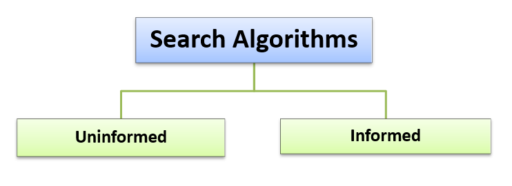
The uninformed search algorithms are unaware of the domain knowledge like the closeness, the goal location. It only knows how to traverse and how to distinguish between a leaf node and goal node and hence it is operated in a brute-force way and so it is also called brute-force algorithms. It searches every node without any prior knowledge and is hence also called blind search algorithms.

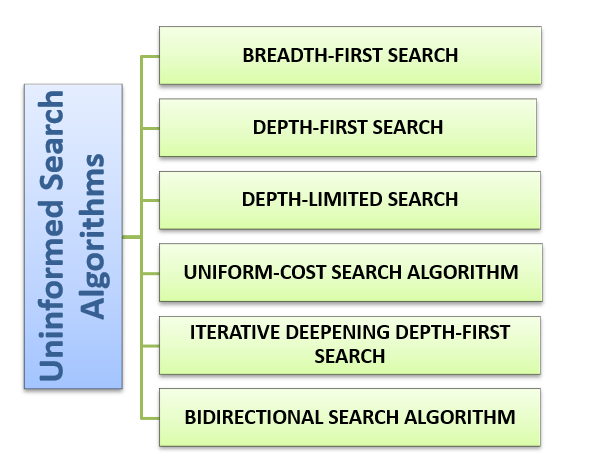
Uninformed search algorithms can be divided into six main types:

1.    BREADTH-FIRST SEARCH:

It is the most common searching strategy to traverse a tree or a graph. It uses a breadthwise searching procedure and hence it is called breadth-first search. The process starts from the root node of the tree and expands to all the successor nodes at the first level before moving to the next level nodes. The queue data structure that works on the First In First Out (FIFO) concept is used to implement this method. As it returns a solution (if it exists) it can be said as a complete algorithm.

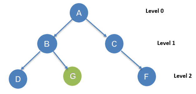
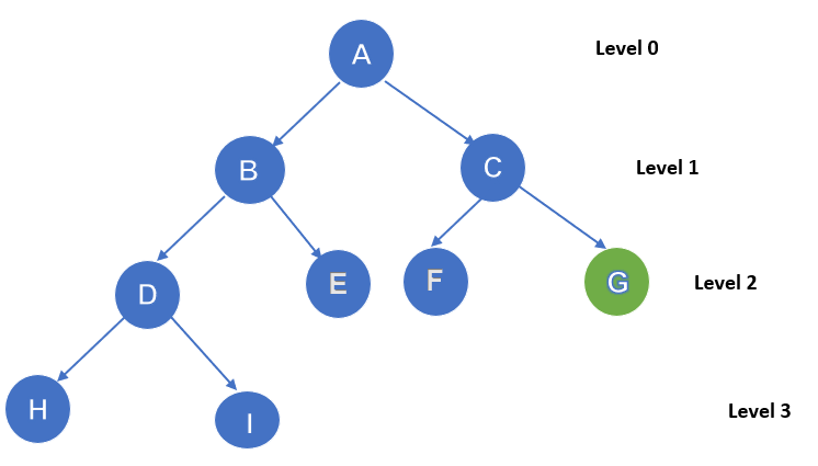
The searching procedure starts from the root node A. Here the goal node is G. from node A it will traverse in an order of A-B-C-D-G. it will traverse level-wise.

Advantages	Disadvantages
Provides a solution if any exist. A minimal solution with the least number of steps is provided when there exists more than one solution for a given problem.	Increased memory requirement since each level of the tree must be saved in the memory to expand the next. Time requirement is more if the solution is far from the root node.

2.    DEPTH-FIRST SEARCH:

It is a process similar to that of BFS. The searching procedure starts from the root node and follows each path to the greatest depth and then backtracks before entering the next path. The stack data structure that works on the concept of Last In First Out (LIFO) is used to implement the procedure.
Example: 

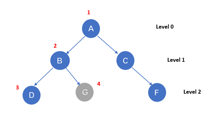
The searching procedure starts from the root node A. Here the goal node is G. From node A it will traverse in an order of A-B-D-G. it will traverse depth-wise.

Advantage	Disadvantage
Less space requirement because it stores nodes linearly. The time requirement is less than BFS.	The algorithm may go in an infinite loop. Possibility of re-occurrence of states.

 

3.    DEPTH-LIMITED SEARCH:

It is much similar to a depth-first search with a predetermined limit. The main disadvantage of DFS is the infinite path, this can be solved with a Depth-limited search. Here the node at the limit is treated like it has no successor nodes further. It can be called an extended and refined version of DFS.

Depth-limited search will terminate with two conditions.

• Standard failure value: Indicates that the given problem doesn’t have any solution
• Cutoff failure value: indicates that there is no solution for the given problem within the given limit.

Example :

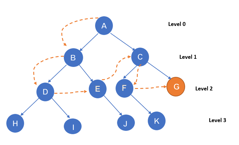
The searching starts from node A. The limit for the procedure is set as l=2. Our goal state is node G. The process is like A-B-D-E-C-F-G.

Advantage	Disadvantage
Memory efficient	Incompleteness Not optimal for problems with more than one solution.

 

4.    UNIFORM-COST SEARCH ALGORITHM:

It is used to traverse a weighted tree or graph. It is different from both DFS and BFS. Here the cost is considered as factor. There is more than one path to reach the goal. The path with the least cost is selected. For traversing the path an increased order of cost is selected.  If the cost is the same for each transition then it can be said to be similar to that of BFS.

Example.

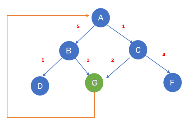
If the starting node is A and the goal to reach is G, then it will traverse A-C-G. The cost will be 3

Advantage	Disadvantage
Optimal because the least cost path is chosen.	May be stuck in an infinite loop because the path cost is only considered.

 

5.    ITERATIVE DEEPENING DEPTH-FIRST SEARCH:

It is a combination of both DFS and BFS. It will find the best depth limit and the limit is gradually increased until a goal is found. The algorithm performs a depth-first search to a certain depth limit and this depth limit is increased after each iteration until the goal is reached. The fastness of BFs and the memory efficiency of DFS are combined within this iterative deepening depth-first search. With large search space and unknown depth of the goal node, this can be more useful.

Example:

1’st Iteration------A
2’nd Iteration------A,B,C
3’rd Iteration------A,B,D,E,C,F,G
4’th Iteration------A,B,D,H,I,E,C,F,K,G
The goal node is found at the 4th iteration.
 

Advantage	Disadvantage
Fast search Memory efficiency	Previous works are repeated.

 

6.    BIDIRECTIONAL SEARCH ALGORITHM:

It performs two searches simultaneously. One from the starting end is called forward-search and the other from the end is called backward search. One single graph is replaced with two small subgraphs one from the initial vertex and the other from the final vertex. The searching procedure stops when these two graphs intersect each other. It can use search techniques such as BFS, DFS, DLS, etc.

Example:

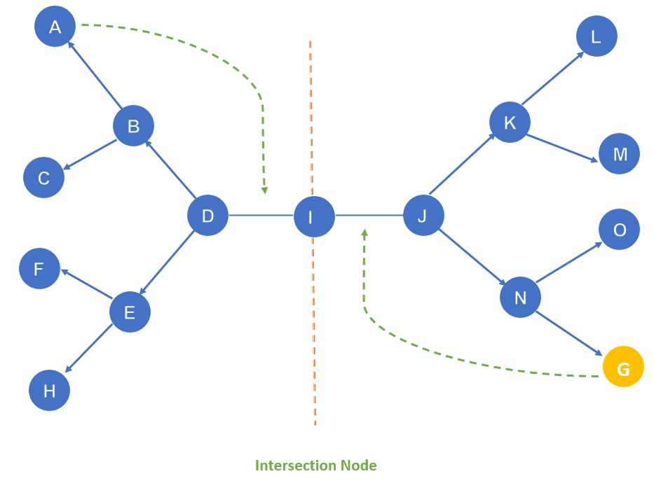
The algorithm terminates at node I where the two sub-graphs meet.

Advantage	Disadvantage
Fast Less memory	Implementation is difficult The goal state must be known.