Discriminant Analysis

---

---

We found that logistic regression is a useful algorithm for binary classification by mapping the linear relationship between the log odds of a class and the data. However, logistic regression is still limited by linear assumptions. 

In this tutorial, we’ll discuss discriminant functions: functions that try to identify which combination of variables can separate out multiple classes. 

Limitations of Logistic Regression or Need of Linear Discriminant Analysis

Logistic regression is a strong and powerful classification algorithm that comes under supervised learning. But it has some limitations that made the formation of LDA and other algorithms

1. Binary Problem:  As we know the logistic regression is very effective in binary classification problems. As you know it has multi-class classifications but is not much used.
2. Unstable:  logistic regression is perfect in normal cases but when the classes are perfectly separated than the logistic regression becomes unstable
3. Not Good when there is less data: If the data is not in plenty to estimate parameters, then the logistic regression may cause some errors and we call it not stable.

LDA solves these problems and can be used instead of logistic regression if there are any of these conditions. IT will be good if you try both and select the best one.

Linear Discriminant Analysis

Linear discriminant analysis(LDA) is a method, which is used to reduce dimensionality, which is commonly used in classification problems in supervised machine learning. It is used for projecting the differences in classes. In simple words, we can say that it is used to show the features of a group in higher dimensions to the lower dimensions.

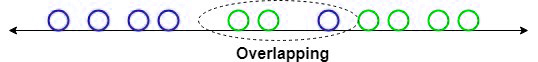
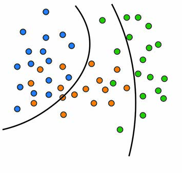
Suppose we have two groups of different data with different features and we want to separate them or classify them using a single feature. When we are doing so, there may be a high chance of overlapping as shown in the picture. So we have to increase the number of features for having a good classification.
 

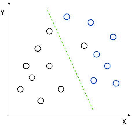
Consider an example for making the concept more clear. Let us have two set of data which are of different groups. Now we want to categorize them into two different groups as in the 2D picture. But when we try to make the data points in a 2D graph, there will not be a linear line to separate the data into two groups.

In such cases we uses the linear discriminant analysis that reduce the 2D graph in to single dimension graph so we get more seperatability between the data points in two groups.

In this method, the LDA is using the graph coordinates such as X-axis and Y-axis to create a new coordinate and show the data using the new coordinate or axis. So we achieve the single dimension reduction from a 2D graph and helps to increase the separation.

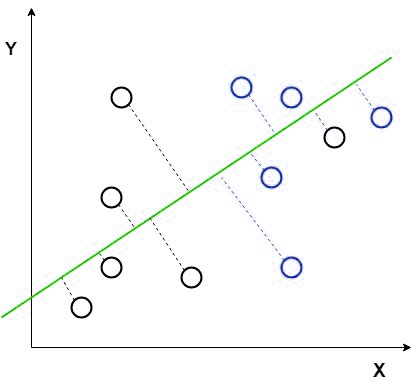
The new cordinate is made using two rules that are

• Increase the distance between the mean of two groups to maximum
• Decrease the variance of two groups to minimum.

In the above picture we shown the new axis in red color and we have plotted the data points with respect to new axis such  that the distance between the mean of two group is increased and the variance between the two groups are reduced. 

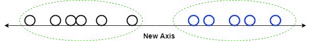
After plotting the datapoints using our rules on the new axis it will be like this as in the below picture.

The function above is the discriminant function, which tells us how likely a data point belongs to class k. Note that π_k is the prior for class k and that f_k is the probability density function of the data for class k. 

For LDA, we’ll assume that the data is a Normal distribution with a mean μ_k. We’ll also assume that the covariance matrix Σ is the same across all classes. Thus, we obtain the following discriminant function:
 

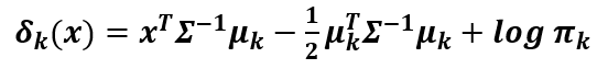
The main point is this: if we compare any two classes, the line that best separates the two classes is a linear function. Thus, LDA finds the best lines that separate any two classes.

We can’t able to use this linear discriminant analysis all time as it will get fail if the mean is shared as the LDA can’t able to find the new coordinate and the axis. In that case, we use nonlinear discriminant. Some popular examples for the nonlinear discriminant are

1. Quadratic Discriminant Analysis: In this method, every class has its own estimate of variance. Or the covariance if there are more than two inputs.
2. Flexible Discriminant Analysis: It will be used in the splines which we discussed in the previous tutorial as the inputs are nonlinear combinations
3. Regularized Discriminant Analysis: we know what is regularization is and in this method we introduce the regularization in the estimation of variance. Which helps the variable influence on LDA will be reduced.

Quadratic Discriminant Analysis

Now, what if we wanted to find curves that can separate more non-linear data? To do this more complex task, we need to determine and consider the differences in variances for each class. 

If we don’t assume that the variance is the same for each class, the discriminant function becomes more complex:

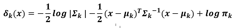
The takeaway is that by not assuming equal variance, the discriminant function becomes a quadratic function. This allows us to separate non-linear data with unequal variances.

When to choose linear versus quadratic discriminant analysis?

Discriminant analysis is useful for classifying data using linear and nonlinear decision boundaries, but there are specific cases where you would want to use one algorithm over another. 

The following table describes use-cases for choosing between linear and quadratic discriminant analysis.

	LDA	QDA
# of observations	Low	High
# of features	High	Low
Data distribution	Normal	Nonlinear