Regression: Linear Regression

What is Linear Regression?

Linear regression is a method to model the relationships between features called independent variable or input variables and the response or the output, which are dependent variables to a set of input features. 

Linear regression is one of the most common and popular machine-learning algorithms for regression analysis. Linear regression uses statistical methods and the output will be real and continuous which is used for the prediction of sales, age, product price expectations, etc.

 The main assumption this method uses is that the parameters or coefficients that the model aims to learn are straight lines. 
 

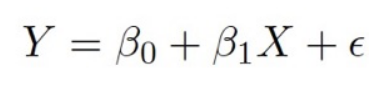
A simple example is shown below:

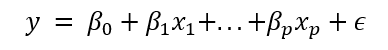
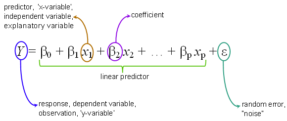
Where p is the number of predictors in the dataset, β₀ is the intercept and β_p represents the parameter we’re trying to estimate with a given feature xp.

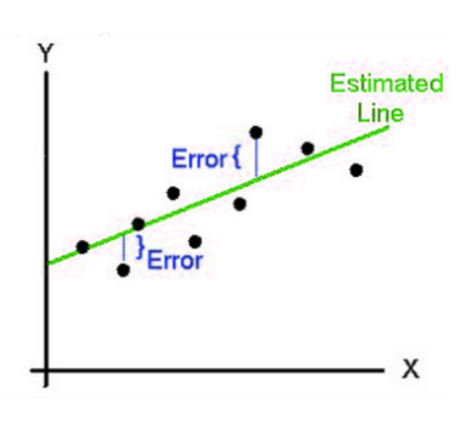
ε is the residual: how far off the line is from the actual datapoint. This variable is important because it is a measure of how erroneous a model is. The squared-sum of the residuals or RSS is a metric used to evaluate the fit of the model. 

Linear regression will help to visualize the relation between the input variable and the prediction output, which will be linear, means straight lines hence, we call it linear regression.

In a graphical representation of linear regression, the independent input variable will be on the X-axis and dependent output will be on the Y-axis and the linear regression will be a sloped straight line connecting maximum data points.
 

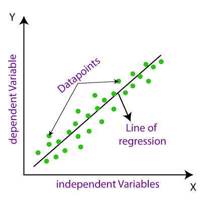
In this graphical representation, we can understand how the linear regression is shown as a straight line with maximum data points connected.

What makes a model linear?

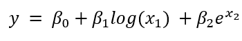
Note that while the relationship between the model parameter β and the predictor x needs to be linear, non-linear functions can be applied to the data. The following equation would be considered to be a linear regression problem, despite being more complex:

What makes a model non-linear?

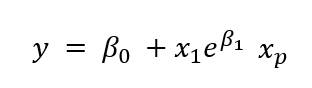
The following equation is a nonlinear function, as the parameter is not proportional to the predictor. 

What are the types of linear regression?

In the regression analysis tutorial, we already told the linear regression can be divided into two again as 

1. Simple linear regression
2. Multiple linear regression

Simple Linear Regression

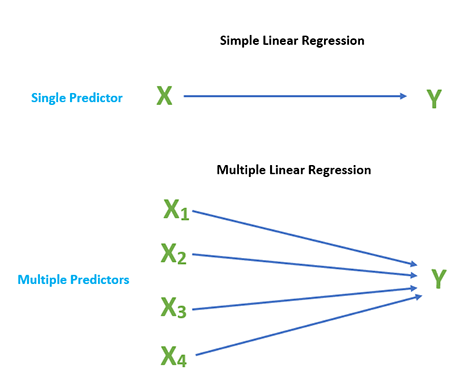
If we have only one independent input variable for determining the output we call such machine learning algorithms as simple linear regression.

We can say this in a simple line as

• Y represents the Predicted output or dependent variable.
• β0 is a constant that represents the intercept (estimate of regression)
• and β1 is a constant that represents coefficient (estimate of regression slope).
• ε (Epsilon) is the error term.

In this graphical representation, we can understand how the simple linear regression is shown as a straight line with data points connected.

Multiple linear regression

Multiple linear regression is the opposite of simple regression as if we have more than one input predictor variable for determining the dependent output variable we call such machine learning algorithms as multiple linear regression. The input variables can be continuous or categorical.

The equation that describes how the predicted values  are related to independent variables in the Multiple Linear Regression equation 

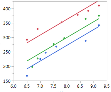
The above graph shows Plotting Multiple linear regression lines on one graph

What is a linear regression line?

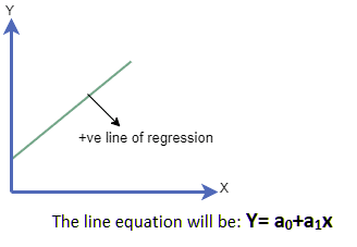
In a linear regression graph, we know there is a straight line that relates the relationship between the input variable and the predicted variable which is called the linear regression line. In this graph linear regression line can show us two different relations which are,

1. Positive Linear relation

   In the linear regression graph if both the input independent variable and the predicted output variable is increasing along the x and the Y axis respectively is called positive relation.

   

2. Negative Linear relation

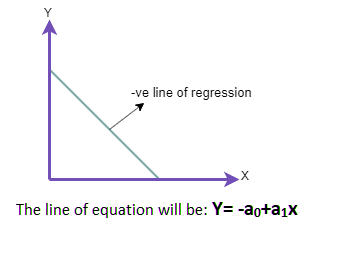
   In the linear regression graph, if the input variable is increasing along the x axis and the predicted output variable that is depended on independent input variable is decreasing along the Y axis and the regression line will meet the y axis at some point. Is called Negative linear relation.

   

Model Performance

Model performance can be described as how the line of regression relates with the data points, how much they touch, and how much distance from the regression line. We have to find the best model from the different models we have in regression is called optimizing the model that can be done as

R –Squared Method

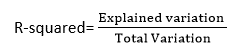
It is a simple statistical method to determine how the regression line fits with the data points in the graph. How the R squared method works is it calculates the relationship strength of the input and the output variables on a 10 to 100--percentage scale.

The value of the R square method is used to determine the model's perfection. A high value for R means the model is good because it says there is less difference between the predicted values and real values. This is also called as the coefficient of determination.

We can calculate the R square value using the formula 

Least-Squares Regression

The most common method for training a regression model is the least-squares method. This model aims to minimize the sum of the square errors from each data point to the line that represents the relationship between x and y.

Mathematically, we can write this relationship as the following statement:

Important notes about the mathematical notation:

• This shorthand notation shows that β is a vector of 1 x the number of features in the dataset. 
• If the features occupy the columns, X^T is a matrix with n observations by m features. 
  • We need to transpose the dataset (flip the rows and columns) to make the mathematics work. 
• The intercept β⁰ can be a scalar or vector.

Why Perform Least-Squares Regression?

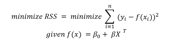
The least-squares regression is a relatively simple model. We’re trying to find the line that best fits the data while minimizing the error of our model. 

So why would we want to use least squares with real data?

1. It’s simple and fast to implement, which is advantageous if we need a fast model
2. It’s interpretable and easy to diagnose for errors: the relationship between the inputs and outputs is clearly defined. 
   • If there are issues in the data such as outliers, least-squares would be able to help us troubleshoot some of those obvious abnormalities. 
3. It’s the worst-case scenario: we know that more complex models would outperform least-squares, especially if the data contained nonlinear relationships. 
   • However, the predictions from least-squares can act as a worst-case scenario for our modeling approach.
      

Assumptions with Least-Squares Regression

• In order to use linear regression, we must assume several things to ensure that we are getting the best results we can. This includes assuming that:
• The relationship between x and y is linear.
• The data is free of outliers and noise.
• The data has been filtered so that highly correlated features are removed. These kinds of features are collinear and will cause the linear model to overfit the data.
• The data structure is Normal data distribution.

Implementing linear regression in Python: The Boston House Price Dataset

Description of the Data

The Boston Housing Dataset is a classic dataset that contains several features associated with the Boston housing market, including crime rate and median value of homes in 1978.

The problem we are solving

The goal of this dataset is to predict the median price of a home. 

We’ll set the features and the target dataset to be a Pandas data frame datatype to be easier for analysis downstream.

# Import general-use data science libraries
import pandas as pd
import numpy as np

# Import features
df = pd.DataFrame(data=data.data, 
                  columns=data.feature_names)
print(df)

# Import target (median housing prices)
target = pd.DataFrame(data=data.target, 
                      columns=["MEDV"])
print(target)
 

 CRIM    ZN  INDUS  CHAS    NOX  ...  RAD    TAX  PTRATIO       B  LSTAT
0    0.00632  18.0   2.31   0.0  0.538  ...  1.0  296.0     15.3  396.90   4.98
1    0.02731   0.0   7.07   0.0  0.469  ...  2.0  242.0     17.8  396.90   9.14
2    0.02729   0.0   7.07   0.0  0.469  ...  2.0  242.0     17.8  392.83   4.03
3    0.03237   0.0   2.18   0.0  0.458  ...  3.0  222.0     18.7  394.63   2.94
4    0.06905   0.0   2.18   0.0  0.458  ...  3.0  222.0     18.7  396.90   5.33
..       ...   ...    ...   ...    ...  ...  ...    ...      ...     ...    ...
501  0.06263   0.0  11.93   0.0  0.573  ...  1.0  273.0     21.0  391.99   9.67
502  0.04527   0.0  11.93   0.0  0.573  ...  1.0  273.0     21.0  396.90   9.08
503  0.06076   0.0  11.93   0.0  0.573  ...  1.0  273.0     21.0  396.90   5.64
504  0.10959   0.0  11.93   0.0  0.573  ...  1.0  273.0     21.0  393.45   6.48
505  0.04741   0.0  11.93   0.0  0.573  ...  1.0  273.0     21.0  396.90   7.88

[506 rows x 13 columns]
     MEDV
0    24.0
1    21.6
2    34.7
3    33.4
4    36.2
..    ...
501  22.4
502  20.6
503  23.9
504  22.0
505  11.9

Split the data into training and test sets

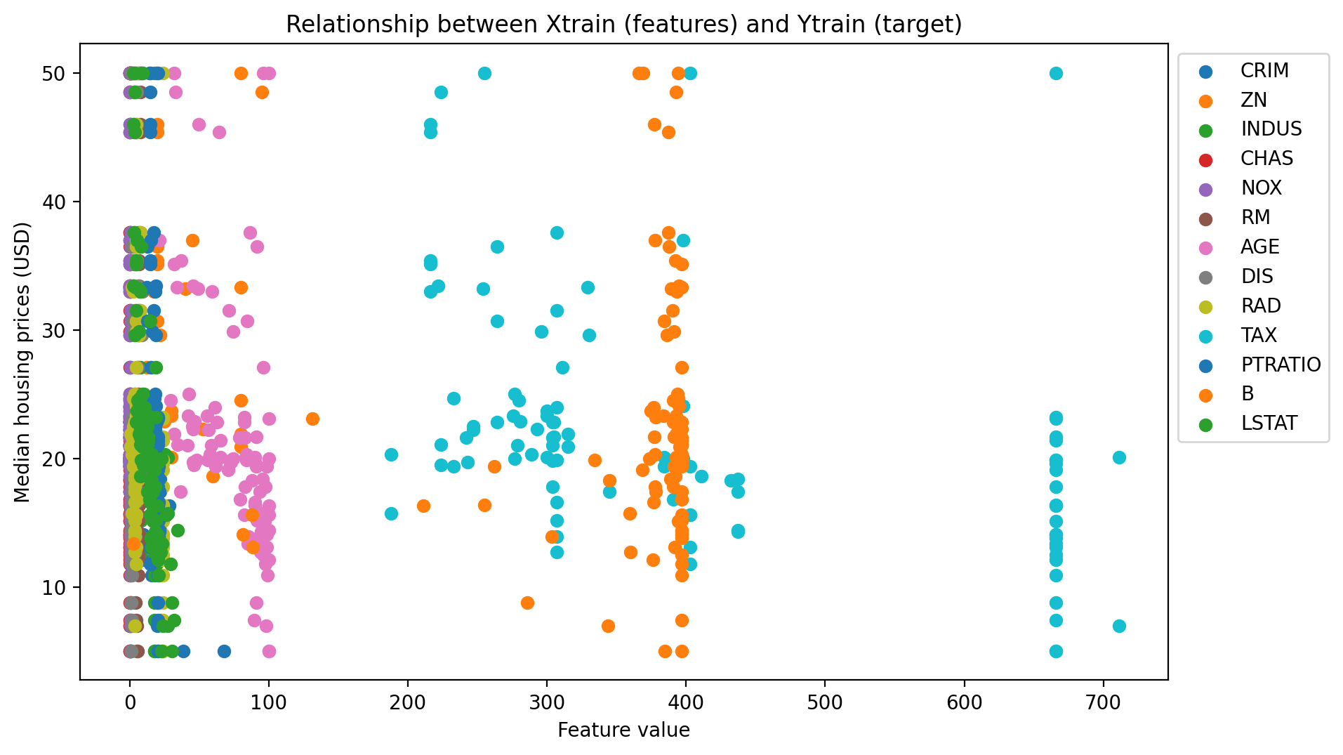
from matplotlib.pyplot import figure
fig, ax = plt.subplots()
for i in Xtrain:
  plt.scatter(Xtrain[i], Ytrain, label=str(i))
ax.legend(bbox_to_anchor=(1., 1.))
plt.xlabel("Feature value")
plt.ylabel("Median housing prices (USD)")
plt.title("Relationship between Xtrain (features) and Ytrain (target)")
fig.set_dpi(200)

savepath="/content/img/"
fig.set_size_inches(10, 6)
fig.savefig(savepath+"scatter.png", bbox_inches='tight')
 

Dataset sizes after train_test_split()
Xtrain size:  (101, 13)
Xtest size:  (405, 13)
Ytrain size:  (101, 1)
Ytest size:  (405, 1)

Visualize the data

from matplotlib.pyplot import figure
fig, ax = plt.subplots()
for i in Xtrain:
  plt.scatter(Xtrain[i], Ytrain, label=str(i))
ax.legend(bbox_to_anchor=(1., 1.))
plt.xlabel("Feature value")
plt.ylabel("Median housing prices (USD)")
plt.title("Relationship between Xtrain (features) and Ytrain (target)")
fig.set_dpi(200)

savepath="/img/"
fig.set_size_inches(10, 6)
fig.savefig(savepath+"scatter.png", bbox_inches='tight')
 

Training A Linear Regression

# Fit the model
from sklearn.linear_model import linear_model as lm
model = lm().fit(Xtrain, Ytrain)
print(model)
 

LinearRegression(copy_X=True, fit_intercept=True, n_jobs=None, normalize=False)

Examine model components 

print("Important model objects")
print("Regression coefficients: ", str(model.coef_))
print("Y-intercept: ", str(model.intercept_))
 

Important model objects
Regression coefficients:  [[-1.10998550e-01  5.59525865e-02  1.52041041e-01  1.62336940e+00
  -2.52970054e+01  3.14436742e+00  3.94375733e-02 -1.31328247e+00
   3.01518760e-01 -1.20457172e-02 -1.23308582e+00  6.49058329e-03
  -6.06938545e-01]]
Y-intercept:  [47.50246908]

Evaluate model

There are several methods that are associated with the model object. If we wanted to make a prediction with the test set, we can use the predict() method.

Ypred = model.predict(Xtest)
print(Ypred)
 

[21.04711236]
 [16.0519687 ] 
 [22.08124826]
 [24.9550908 ]
 [22.58486361]
 [18.30309637]
 [36.34589925]
 [20.84835474]
 [34.53960168]
 [25.75900913]
 [18.57619619]
 [ 3.15134125]
 [24.60956537]
 [18.28628001]
 [15.22482753]
 [29.71273752]
 [31.22651416]
 [22.66172954]
 [20.61047944]
 [22.90176779]
 [26.96548001]
 [19.92578633]
 [31.0290531 ]
 [19.55288498]
 [19.0799543 ]
 [23.47680399]
 [18.14110649]
 [14.52089098]
 [27.04951364]
 [25.58432198]
 [22.15694304]
 [21.72038631]
 [20.88291021]
 [18.1170226 ]
 [19.05318278]
 [30.97678281]
 [30.5478923 ]
 [16.62990827]
 [18.75101055]
 [33.66266989]
 [17.01643957]
 [14.17095253]
 [32.62854346]
 [24.94957009]
 [13.37233271]
 [24.45143619]
 [20.09491092]
 [38.58474904]
 [44.15771256]
 [21.54061052]
 [21.61272714]
 [ 3.85894539]
 [19.81522043]
 [42.8604927 ]
 [26.02782308]
 [35.09436136]
 [23.79821583]
 [18.26944428]
 [32.92705099]
 [14.8280985 ]
 [20.77294734]
 [12.31289156]
 [34.24357418]
 [22.66837597]
 [13.22221194]
 [21.63774045]
 [17.37198566]
 [17.85270836]
 [30.28365937]
 [32.18075657]
 [20.45336081]
 [29.75959666]
 [ 7.18982288]
 [18.89723132]
 [30.10475681]
 [20.57839242]
 [33.3974039 ]
 [24.24358861]
 [14.26738546]
 [24.20106907]
 [32.91401148]
 [17.80684621]
 [26.29527134]
 [22.10605813]
 [24.43018928]
 [32.65649583]
 [26.2304317 ]
 [23.11068013]
 [21.37121057]
 [21.59383797]
 [11.26008499]
 [16.94212371]
 [22.85497267]
 [29.61466174]
 [23.09151181]
 [12.26582213]
 [24.38136745]
 [13.14379108]
 [ 7.98377975]
 [31.77241579]
 [12.00109812]
 [13.18440467]
 [31.33628903]
 [19.70216857]
 [28.20054128]
 [ 0.60101149]
 [31.12712135]
 [24.19502058]
 [29.53687253]
 [ 9.68649156]
 [10.11971136]
 [ 7.12036418]
 [20.70524276]
 [14.50594171]
 [23.88299493]
 [22.20130119]
 [ 6.58848017]
 [18.23088525]
 [30.87930596]
 [14.74069658]
 [22.10694463]
 [32.68525461]
 [29.82819265]
 [30.72089238]
 [19.16986842]
 [29.39425529]
 [17.80744526]
 [21.82646237]
 [24.31193619]
 [30.23574889]
 [20.25455558]
 [15.88697828]
 [23.44452457]
 [21.86141303]
 [14.83881915]
 [32.36894068]
 [23.76741903]
 [21.66801612]
 [13.53616923]
 [16.77326467]
 [16.68268242]
 [33.67449135]
 [30.06984231]
 [25.98382116]
 [15.58993356]
 [17.51342189]
 [ 5.72952529]
 [12.49735596]
 [27.35548835]
 [35.55403582]
 [26.03031409]
 [30.2652679 ]
 [20.79109449]
 [13.36025789]
 [25.72460123]
 [ 8.9366379 ]
 [15.54265181]
 [25.21990601]
 [18.55971622]
 [32.15802211]
 [36.40020073]
 [22.56136319]
 [22.7234512 ]
 [34.37231992]
 [-3.94468944]
 [14.23851594]
 [20.31829917]
 [32.69907633]
 [21.14937346]
 [27.1818681 ]
 [20.77005275]
 [26.33401396]
 [18.66135437]
 [29.2236251 ]
 [32.13618142]
 [13.65673552]
 [ 9.83952335]
 [37.20348635]
 [20.45829063]
 [18.82696886]
 [22.46200016]
 [20.70769228]
 [24.98878401]
 [24.94873464]
 [22.63186389]
 [27.95664184]
 [34.95321661]
 [29.57340438]
 [ 6.2979752 ]
 [18.58409807]
 [22.12319937]
 [21.82862584]
 [12.68613277]
 [11.81831775]
 [23.86158832]
 [24.73085406]
 [30.67013986]
 [24.06240533]
 [34.82481321]
 [18.24315249]
 [15.27193751]
 [11.26864556]
 [31.03156474]
 [27.71373401]
 [41.03106415]
 [28.29517411]
 [19.41491991]
 [36.25536337]
 [21.12170882]
 [32.81354451]
 [24.64850689]
 [31.94774974]
 [19.8091977 ]
 [17.03760649]
 [28.82566707]]

Then we can compute the MSE.

mse = np.square(np.mean(Ytest-Ypred))
print(mse)
 

MEDV    0.139942
dtype: float64

If we wanted to get a measure of how well the line fits to the test dataset (a.k.a the coefficient of determination), we can use the score() method.

R2 = model.score(Xtest, Ytest)
print(R2)
 

0.7219648298245812

The coefficient of determination assumes a value between 0 and 1, where 1 is a perfect line fit. We have a pretty good score!