Naive Bayes

---

---

Naïve Bayes is supervised machine learning which is used for solving classification problems. Naïve Bayes is used mainly for the test classification problems and it works using the principle of Bayes theorem.

As we know, supervised machine learning uses the training dataset for training the model, in this method it uses a high dimensional training set. The Naïve Bayes algorithm is simple and very accurate and increases the efficiency of the model that making the model very fast in giving the predictions.

The Naïve Bayes algorithm works on probability and it is called a probabilistic classifier algorithm. Popular examples of the naïve Bayes algorithm are article classifier and spam detection and filtration.

Bayes Theorem

Compared to traditional statistical methods that assume the world works at random, Bayesian statistics aims to model the probability of an occurrence using the knowledge of past events or experiences. 

The take-home point for Bayes’ theorem is that we are trying to estimate the relationship (or probability) of a given class from data, without knowing the causal relationship between the data and class. 

Mathematically, this can be expressed using the following formula, and we'll break these points down in further sections:

The posterior probability (or prediction): P(class | data)

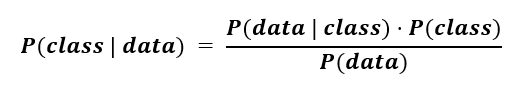
P(class | data)is the probability that the class is associated with a given data set. This is known as a conditional or posterior probability. 

This is the formal definition of what we aim to estimate in a classification problem: we are trying to predict the chances of a data point belonging to a specific class, given some data attributes.

Prior information: P(class)

Now the probability of a given class occurring in the dataset P(class) is relatively easy to estimate - we can see how frequently the class is observed. This term is known as a prior because it is obtained from prior knowledge of the data. 

Likelihood: P(data | class)

Additionally, the probability of the data point is associated with a given class (P(data | class))is also easily obtainable. In this case, we may happen to know certain thresholds for important features that increase the chances of a data point being grouped into a class. This is known as the likelihood.

Evidence: P(data)

Finally, we may (or may not) have information about the distribution of a given feature in the data. This usually needs to be estimated by having a lot of previous examples, as this would provide evidence that our data has a specific form. Nonetheless, we can make assumptions about the data that allow us to make this variable negligible.   

Putting it all together

Now, if we revisit the formula, we can reframe the Bayes theorem using words that will convey some intuition on the mathematics:

While in practice it is difficult to use Bayes’ theorem (because we usually don’t have hard evidence), we can make assumptions that allow us to make a predictive model. One simplification is known as Naive Bayes.

Why it is called the Naïve Bayes algorithm?

So, why is this machine learning algorithm called naïve Bayes? As we know this algorithm is based on the Bayes theorem and that is why it is called the Bayes. Now Naïve means the features are independent of each other.

Suppose we have an orange that has features like color and shape that individually contribute to the features and do not depend on each other.

Naive Bayes 

Naive Bayes uses Bayes’ theorem but makes 1 (naive) assumption to simplify the mathematics: all the features in the training dataset are assumed to be unrelated to each other. 

In other words, each feature is independent of one another and there is no correlation (or anticorrelation) between features.

Why is this important? Since we don’t know the underlying data distribution, and we choose not to acknowledge it, we can ignore the denominator. Thus, the calculation simplifies into an additive formula, where we are summing the contribution of each p feature to the likelihood of observing a given class k:

Note: this means that each feature in the data has some predictive relationship to a given class, and this relationship is assumed to be independent of the other features in the data. While this is not true in all real-world datasets, this method surprisingly works well with high accuracy! 

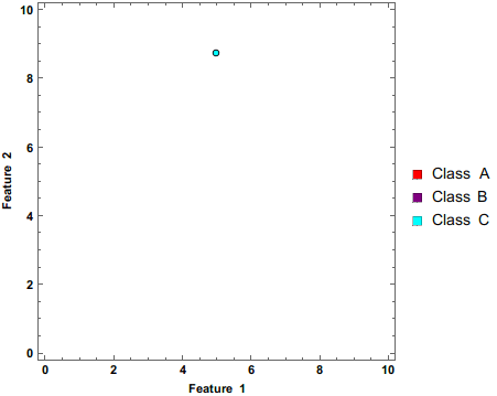
Shown above is a Naive Bayes classifier working to separate 3 classes as additional data points are being added. Note that the circles have darker colors. This shows that these predictions are being made based on probabilities.  

Working of Naïve Bayes algorithm

We can check the working of the naïve Bayes algorithm using a simple example, which makes it easy to understand. Suppose we have some data about the weather and we need a prediction about whether we can go out on a particular day depending upon the weather conditions. For that we have to do some steps for the proper predictions
1.    We have to convert the given dataset into frequency tables
2.    Generate a table by using the probability for rain using weather data
3.    Use the Bayes theorem to predict the output

Now we have a problem: can we go out if the weather is sunny? 

For getting a solution for that we have to check the below tables

	Outlook	Play
0	Rainy	Yes
1	Sunny	Yes
2	Cloudy	Yes
3	Cloudy	Yes
4	Sunny	No
5	Rainy	Yes
6	Sunny	Yes
7	Cloudy	Yes
8	Rainy	No
9	Sunny	No
10	Sunny	Yes
11	Rainy	No
12	Cloudy	Yes
13	Cloudy	Yes

Now we have a table depend on the frequency on weather conditions

Weather	Yes	No
Overcast	5	0
Rainy	2	2
Sunny	3	2
Total	10	5

 

Then the likelihood table of weather will be like

Weather	No	Yes
Overcast	0	5	5/14= 0.35
Rainy	2	2	4/14=0.29
Sunny	2	3	5/14=0.35
All	4/14=0.29	10/14=0.71

After getting the table ready we have to apply the bayes theorem for the prediction.

P(Yes|Sunny)= P(Sunny|Yes)*P(Yes)/P(Sunny)
P(Sunny|Yes)= 3/10= 0.3
P(Sunny)= 0.35
P(Yes)=0.71
So P(Yes|Sunny) = 0.3*0.71/0.35= 0.60

P(No|Sunny)= P(Sunny|No)*P(No)/P(Sunny)
P(Sunny|NO)= 2/4=0.5
P(No)= 0.29
P(Sunny)= 0.35
So P(No|Sunny)= 0.5*0.29/0.35 = 0.41

From the calculations above P(Yes|Sunny)>P(No|Sunny) 
That means we have the predictions that we can go out on a sunny day.

Advantages of Naïve Bayes 

• As we told it is a simple and fast machine learning algorithm
• It will be applicable to both binary and multiclass
• It will make good and accurate predictions in the case of the multi-class dataset.
• It can be used perfectly for text classifications

Limitations of Naïve Bayes

•  In the section why the name naïve Bayes we told that it thinks all the features are independent so it cannot find relationships in the features.

Applications of Naïve Bayes

• Helps in real-time predictions
• It can be used for spam filtering
• Used in the medical field
• Helpful in credit scoring

Types of Naïve bayes Models

Naïve Bayes algorithms are of three types, which are

1. Gaussian: it is a method where the model assumes the features are of normal distribution. Which means if the output takes values, which are continuous? The model thinks it will be a Gaussian distribution.
2. Multinomial: If the data is distributed multinomial, we will use the multinomial naive Bayes model and it is mainly used in text classifications.
3. Bernoulli: Bernoulli classifier is similar to the multinomial but the difference is the output variables are independent binary variables. It is used for detecting whether a word is present in a document or not.