

We already discussed the overfitting problem of a machine-learning model which makes the model inaccurate predictions. It will affect the efficiency of the model.
Regularization is the answer to the overfitting problem. We can say that regularization prevents the model overfitting problem by adding some more information into it.
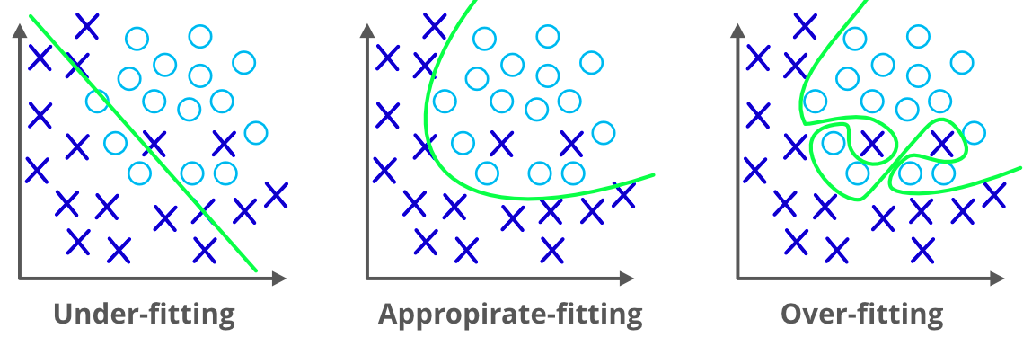
Before going forward we need to know what the overfitting problem is. It happens when a machine learning model performs well with the training dataset and it fails or causes errors when we use the test dataset. We cannot able to use that model to predict the output of the real-valued input variables. To deal with that problem we can use regularization.
In the regularization method we are using all the features in the model but what we reduce is the magnitude of the features so that it can be a more accurate and more generalized model to give good results. In other words, regularization reduces to the usage of a more complex model so as to reduce the chance for overfitting.
Regularization methods add additional constraints to do two things:
In machine learning, regularization problems impose an additional penalty on the cost function. This penalty controls the model complexity - larger penalties equal simpler models. This allows the model to not overfit the data and follows Occam's razor: the simple model is usually the most correct.
The general form of a regularization problem is shown below:
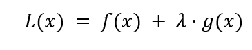
Where f(x) is a loss function (like the residual sum of squares), λ is the regularization term that controls the model complexity, and g(x) is another function that is a function of the regression coefficients.
Different g(x) functions are essentially different machine learning algorithms.
We already discussed the two main techniques used in regularization, which are
Ridge regression is one of the flexible and powerful regression analysis which is used when there is a high correlation between the input variables. If the co-linearity is very high, we will add some bias into the ridge regression method. The amount we add in the bias is called a penalty in ridge regression. Ridge regression has less susceptible to the overfitting problem.
Ridge will help to solve problems with a large number of parameters and have a high correlation between them. Ridge is also used to reduce the complexity of a model that we call L2 regularization.
Ridge Regression is one form of regularization that reduces the impact of correlated features in the dataset. It does that by penalizing larger coefficients, shrinking the coefficients for non-informative specific features.
The mathematical formulation for Ridge regression is shown below:
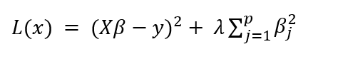
The left-hand term is the residual sum of squares - a measure of the model error against the actual value. The right-hand term is the penalty term. Note that the penalty is a function of β^2, which acts as a constraint for the linear model.
The take-home for Ridge regression is that the model prefers to take smaller β estimates that are close to 0, which reduces the penalty term.
The regularization term λ has a profound impact on model performance and should be selected with care. One method to do that is to simply see how different values for λ model performance.
We'll write up a method to do just that using cross-validation, an essential strategy for evaluating models beyond this tutorial's scope.
We’ll use the Boston data described in the linear regression tutorial to predict the median house prices.
First, load the Boston dataset.
# Import the dataset
from sklearn.datasets import load_boston

data = load_boston()
print(data)

# Import general-use data science libraries
import pandas as pd
import numpy as np

# Import features
df = pd.DataFrame(data=data.data,
                  columns=data.feature_names)
print(df)

# Import target (median housing prices)
target = pd.DataFrame(data=data.target,
                      columns=["MEDV"])
print(target)
Then split into training and test sets.
from sklearn.model_selection import train_test_split
Xtrain, Xtest, Ytrain, Ytest = train_test_split(df, target, test_size=0.8, random_state=1)

print("Dataset sizes after train_test_split()")
print("Xtrain size: ", str(np.shape(Xtrain)))
print("Xtest size: ", str(np.shape(Xtest)))
print("Ytrain size: ", str(np.shape(Ytrain)))
print("Ytest size: ", str(np.shape(Ytest)))
Fit the Ridge model with hyperparameter tuning
# Fit the model
from sklearn.linear_model import RidgeCV
import numpy as np
lambdas = np.array([1.e-06, 1.e-05, 1.e-04, 1.e-03, 1.e-02, 1.e-01, 1.e+00, 1.e+01,
      1.e+02, 1.e+03, 1.e+04, 1.e+05, 1.e+06])
ridge_mdl = RidgeCV(alphas=lambdas).fit(Xtrain, Ytrain)
Like the Ridge regression, Lasso regression also used to reduce the complexity of the model by adding some penalty. The only difference is we add the actual amount to a penalty in Lasso, as in ridge we use a square of the amount.
The Least Absolute Shrinkage and Selection Operation (LASSO) is another form of regularization. it allows regression coefficients to shrink all the way to 0. This makes the model more sparse and computationally efficient. . Lasso regression is also called L1 regularization
Additionally, LASSO performs feature selection: features with a coefficient of 0 are essentially ignored.
The mathematical formulation for LASSO is shown below:
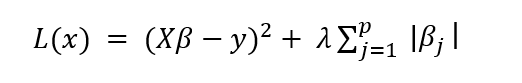
The only thing that has changed from the Ridge formulation is the absolute value in the penalty term.
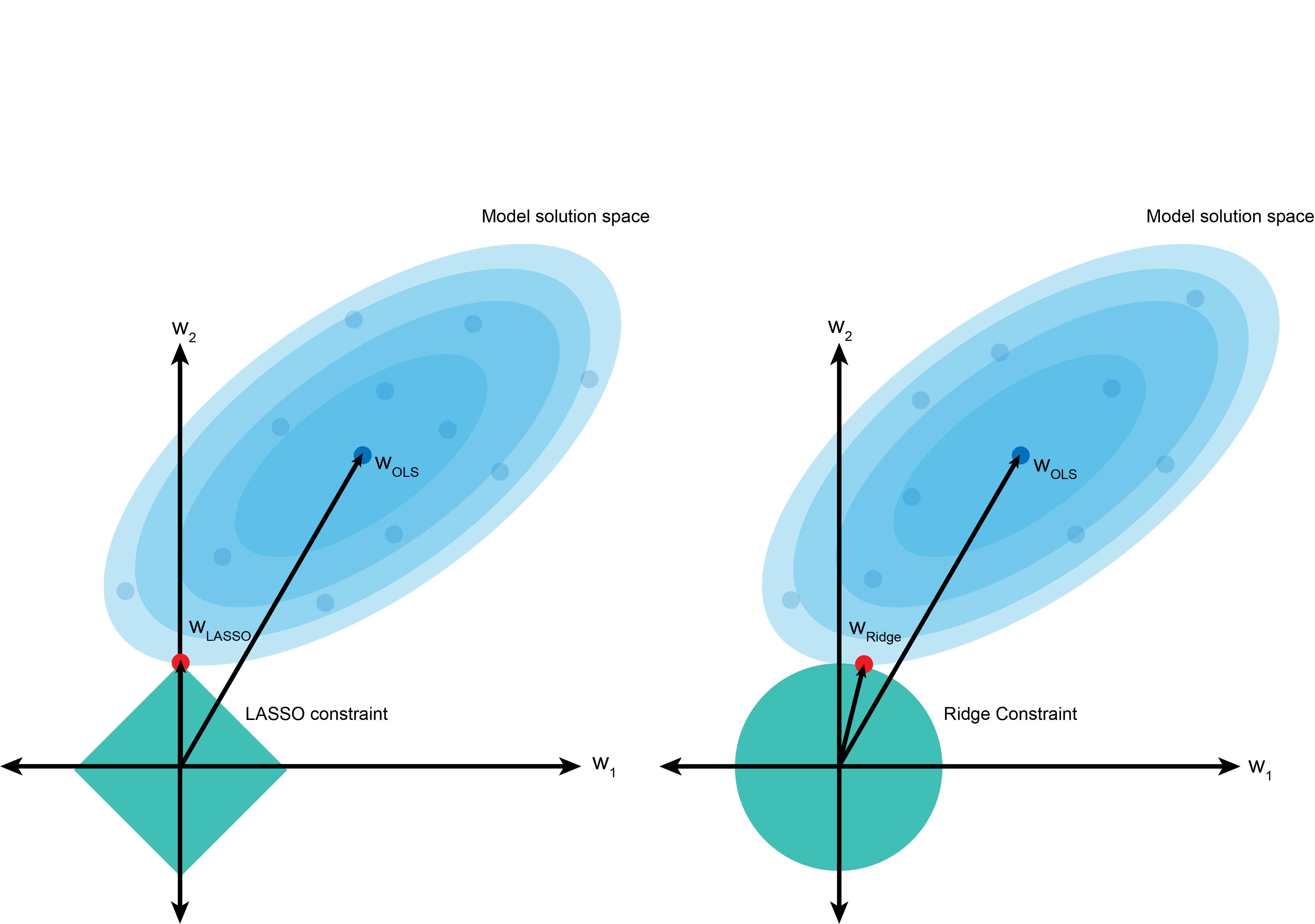
The graph above is a visual representation of LASSO (left) and Ridge (right) regression. The blue cloud represents the least-squares operation, and the center value is the least-squares estimate for β.
However, the penalty term forces us not to take that value and instead choose values in the turquoise boundaries. The square term in Ridge regression results in a circle if we consider a two-dimensional problem (β12+β22). In contrast, the absolute value term in LASSO creates a diamond constraint.
Using the same least-squares model, the circle constraint in Ridge regression makes it likely to shrink the coefficient w2 to be a small value approaching 0 (shown in red), but not necessarily hitting 0. In contrast, LASSO is more likely to penalize the coefficient w2 more harshly and set it to 0 if it is not informative.
As we did with the linear regression and Ridge regression models, we’ll train LASSO on the Boston dataset with hyperparameter tuning.
# Fit the model
from sklearn.linear_model import LassoCV
import numpy as np
lambdas = np.array([1.e-06, 1.e-05, 1.e-04, 1.e-03, 1.e-02, 1.e-01, 1.e+00, 1.e+01,
      1.e+02, 1.e+03, 1.e+04, 1.e+05, 1.e+06])
lasso_mdl = LassoCV(alphas=lambdas).fit(Xtrain, Ytrain)