

The built-in function in the R programming language is the functions that are already existing or pre-defined within an R framework. The built-in functions enable a user or a programmer to program in the R language easily and simpler. R language provides its user with a rich set of pre-defined functions to make their computation more efficient as well as minimize their programming time.
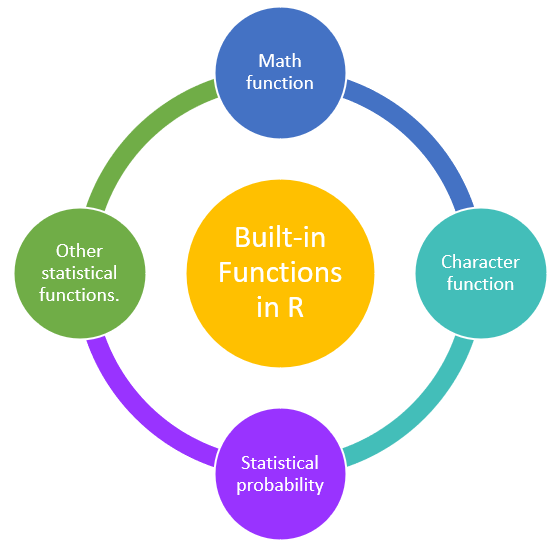
In r programming language the built-in functions are categorized furthers as following
Let us begin exploring the built-in function with some of the Math functions available in The R programming language.
The math function denotes the mathematical or numeric calculations with some built-in functions. The set of instructions for particular functions is predefined in the R program, the user just needs to call the function for accomplishing their task of execution.
The following table highlights some of the numeric or mathematical built-in functions in R.
| Serial No | Built-in function | Description | Example |
|---|---|---|---|
| 1 | abs(x) | It returns the absolute value of input x |
x<- -2 print(abs(x)) Output [1] 2 |
| 2 | sqrt(x) | It returns the square root of input x |
x<- 2 print(sqrt(x)) Output [1] 1.414214 |
| 3 | ceiling(x) | It returns the smallest integer which is larger than or equal to x. |
x<- 2.8 print(ceiling(x)) Output [1] 3 |
| 4 | floor(x) | It returns the largest integer, which is smaller than or equal to x. |
x<- 2.8 print(floor(x)) Output [1] 2 |
| 5 | trunc(x) | It returns the truncate value of input x. |
x<- c(2.2,6.56,10.11) print(trunc(x)) Output [1] 2 6 10 |
| 6 | round(x, digits=n) | It returns round value of input x. |
x=2.456 print(round(x,digits=2)) x=2.4568 print(round(x,digits=3)) Output [1] 2.46 [1] 2.457 |
| 7 | cos(x), sin(x), tan(x) | It returns cos(x), sin(x) , tan(x) value of input x |
x<- 2 print(cos(x)) print(sin(x)) print(tan(x)) Output [1] -0.4161468 [1] 0.9092974 [1] -2.18504 |
| 8 | log(x) | It returns natural logarithm of input x |
x<- 2 print(log(x)) Output [1] 0.6931472 |
| 9 | log10(x) | It returns common logarithm of input x |
x<- 2 print(log10(x)) Output [1] 0.30103 |
| 10 | exp(x) | It returns exponent |
x<- 2 print(exp(x)) Output [1] 7.389056 |
R programming language provides some built-in string or character functions as described in the following table.
| Serial No | Built-in function | Description | Example |
|---|---|---|---|
| 1 | tolower(x) | It is used to convert the string into lower case. | string<- "Learn eTutorials" print(tolower(string)) Output [1] "learn etutorials" |
| 2 | toupper(x) | It is used to convert the string into upper case. |
string<- "Learn eTutorials" print(toupper(string)) Output [1] "LEARN ETUTORIALS" |
| 3 | strsplit(x, split)) | It splits the elements of character vector x at split point. | string<- "Learn eTutorials" print(strsplit(string, "")) Output [[1]] [1] "L" "e" "a" "r" "n" " " "e" "T" "u" "t" "o" "r" "i" "a" "l" "s" |
| 4 | paste(..., sep="") | Concatenate strings after using sep string to seperate them. | paste("Str1",1:3,sep="") [1] "Str11" "Str12" "Str13" paste("a",1:3,sep="M") [1] "aM1" "aM2" "aM3" paste("Today is", date()) [1] "Today is Sun Feb 27 06:26:31 2022" |
| 5 | sub(pattern,replacement, x,ignore.case=FALSE,fixed=FALSE) | Find pattern in x and replace with replacement text. If fixed=FALSE then pattern is a regular expression. If fixed = T then pattern is a text string. |
string<- "You are learning GOlang in Learn eTutorials" sub("GOlang","R",string) Output [1] "You are learning R in Learn eTutorials" |
| 6 | grep(pattern, x , ignore.case=FALSE, fixed=FALSE) | It searches for pattern in x. | string <- c('R','GO','GOlang') pattern<- '^GO' print(grep(pattern, string)) Output [1] 2 3 |
| 7 | substr(x, start=n1,stop=n2) | It is used to extract substrings in a character vector. | string<- "Learn eTutorials" substr(string, 1, 5) substr(string, 4, 10) Output [1] "Learn" [1] "rn eTut" a <- "123456789" substr(a, 5, 3) output [1] "" |
R programming language provides some statistical built-in functions to deal with a probability distribution. Some of the commonly used distribution functions are rnorm, dnorm, qnorm, pnorm. These functions are used to analyze the probability distribution.
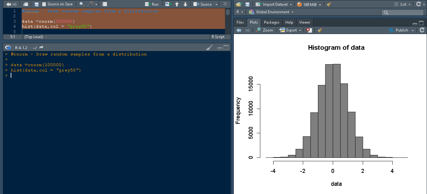
In R programming language rnorm allows drawing random values from a distribution specifically the normal distribution. Let us try drawing 100000 values from the normal distribution and Look at the histogram where values are plotted as shown in the snippet.
#rnorm - Draw random samples from a distribution

data =rnorm(100000)
hist(data,col = "grey50")
The above code shows rnorm() function, the syntax of rnorm is
rnorm(n, mean = 0, sd = 1)
The snippet shows the histogram for the rnorm() created,
This function provides the value of the y-axis corresponding to x-axis in a plot.
dnorm(x, mean = 0, sd = 1, log = FALSE)
Suppose you want to know the value of the y-axis corresponding to a value -2 at the x-axis. By using dnorm(-2) we roughly get the following output
> dnorm(-2)
[1] 0.05399097
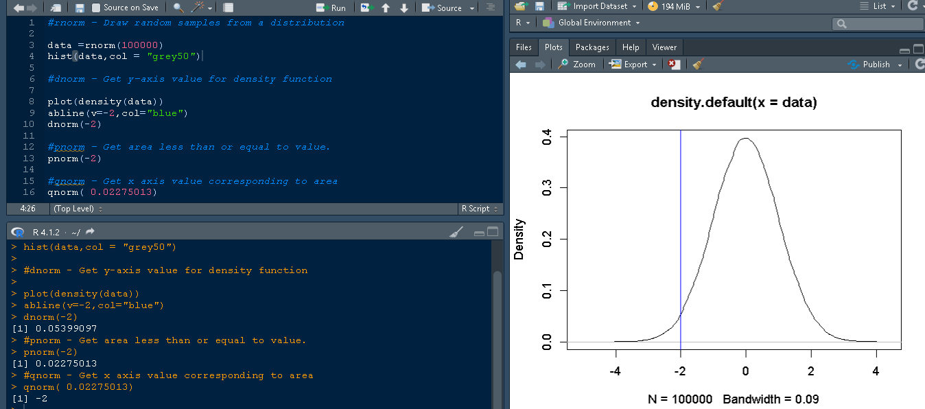
To check the area of a certain value or lower on the curve. Let us plot the density of data to better understand the concept by using the plot() function for the above created data for rnorm.
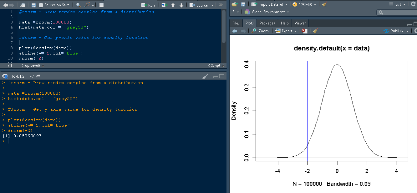
The snippet from RStudio shows the plot corresponding to data with a line on -2 in blue color. In order to know the area under this curve (under -2) use the pnorm function. To find the pnorm of the area underneath -2 use this syntax
pnorm(-2)
It produces an output that indicates the area under the curve or at the blue line is 0.02275013.
> pnorm(-2)
[1] 0.02275013
This function performs just opposite or converse of pnorm(). Consider you want to check an area with a value 0.02275013 you are unaware of the value corresponding to it in the x-axis. This can be accomplished using qnorm function.
qnorm(0.02275013)
Its output return a value -2 corresponding to x axis.
[1] -2
Look at the function pnorm() where we discussed the same points.Both pnorm() and qnorm() are opposites in function.
We need to discuss a lot more under statistical distribution which will be covered in another tutorial. For now, just understand there are certain functions to work with statistical probability distributions.
There are some other functions apart from the above types of statistical functions. The following table describes the additional statistical functions with examples.
| Serial No | Built-in function | Description | Example |
|---|---|---|---|
| 1 | mean(x, trim=0, na.rm=FALSE) |
Calculates the average or mean of a set of numbers Simply calculate mean of object x. | x=c(2,3,4,5) mean(x, trim=0,na.rm=FALSE) Output [1] 3.5 |
| 2 | sd(x) | It returns standard deviation of an object. | x=c(2,3,4,5) print(sd(x)) Output [1] 1.290994 |
| 3 | median(x) | It returns median | x=c(2,3,4,5) print(median(x)) Output [1] 3.5 |
| 4 | range(x) | It returns range | x=c(2,3,4,5) print(range(x)) Output [1] 2 5 |
| 5 | sum(x) | It returns sum. | x=c(2,3,4,5) print(range(x)) Output [1] 14 |
| 6 | diff(x, lag=1) | It returns differences with lag indicating which lag to use. | x=c(2,3,4,5) print(diff(x,lag=1)) x=c(2,3,4,5) print(diff(x,lag=2)) x=c(5,10,15,20,25,30) print(diff(x,lag=2)) Output [1] 1 1 1 [1] 2 2 [1] 10 10 10 10 |
| 7 | min(x) | It returns minimum value of object. | x=c(5,10,15,20,25,30) print(min(x)) Output [1] 5 |
| 8 | max(x) | It returns maximum value of object. | x=c(5,10,15,20,25,30) print(max(x)) Output [1] 30 |
| 9 | scale(x, center=TRUE, scale=TRUE) | Column center or standardize a matrix. | x = matrix(1:15, nrow=3, ncol=5,byrow =TRUE) print(x) Output [,1] [,2] [,3] [,4] [,5] [1,] 1 2 3 4 5 [2,] 6 7 8 9 10 [3,] 11 12 13 14 15 print(scale(x, center=TRUE, scale=TRUE)) Output [,1] [,2] [,3] [,4] [,5] [1,] -1 -1 -1 -1 -1 [2,] 0 0 0 0 0 [3,] 1 1 1 1 attr(,"scaled:center") [1] 6 7 8 9 10 attr(,"scaled:scale") [1] 5 5 5 5 5 |