Factors in R

In our last tutorial, we discussed and learned about data frames in R. In this tutorial you will learn a special data structure known as Factors. One of the most important uses of factors is in statistical modeling.

One who has a statistical background may know about categorical variables. Categorical variables are unlike numerical variables, they can take up only a limited number of different values. Otherwise categorical variables can only belong to a limited number of categories. For example, Yes or No, True or False, Male or Female are some kind of categorical variables in data analysis.

R is a programming language that supports a particular data structure called Factor. When you store categorical data as factors you can assure that all the statistical modeling techniques will handle such data efficiently.

What are categorical variables?

You need to understand categorical variable concepts before moving into our tutorial Factor in depth. You are familiar with the word dataset, a data set is a collection of data. R programming language uses datasets to handle, store and analyze data for data analysis and statistical modeling. These datasets contain mainly two types of variables such as

• Continuous variables
• Categorical variables

A Continuous variable is a variable whose value is unlimited or infinite. In other terms, they contain an uncountable set of values. For example Temperature, the Number of stars in the galaxy, our body weight, are continuous variables. It can take up any value specified between an interval.

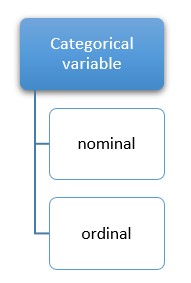
A categorical variable or discrete variable is a variable whose value is finite or contains a distinct group. It means they contain a set of finite values that may have two or more categories (values). There are two types of categorical variables, nominal and ordinal.

1. Nominal variable: - In the nominal variable, there is no intrinsic ordering to its categories. eg: Gender
2. Ordinal variable: - An ordinal variable is just the opposite of a nominal they do have a specific ordering of categorical values. Eg: Temperature.

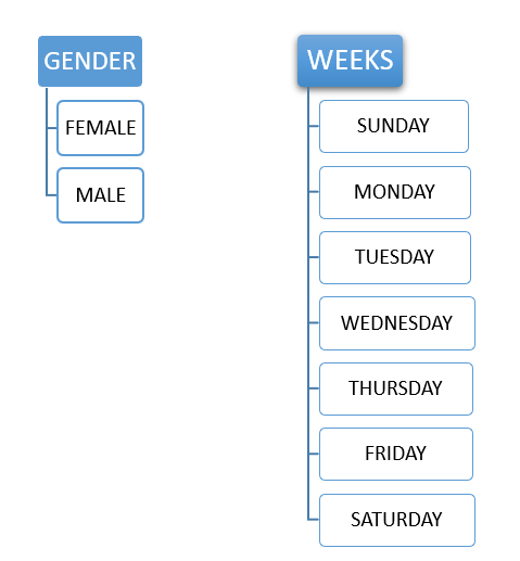
Consider GENDER it forms a nominal categorical variable because it can have only two possible values or categories like MALE or FEMALE. There are no ordering constraints either of the values male or female can be ordered in the first position followed by the next. Likewise, consider WEEKS, weeks can have only 7 values or categories such as SUNDAY, MONDAY, TUESDAY, WEDNESDAY, THURSDAY, FRIDAY, SATURDAY.

TEMPERATURE can be categorized into three LOW, MEDIUM, and HIGH. It falls under the ordinal category. There is a particular ordering for values that begins with low temperature, then medium, and finally reaches a high temperature.

Understanding categorical variables is a basic part before learning Factor in R programming. In the next session, we are going to start with our new data structure.

What are the factors in R?

A factor is a special kind of data structure in R programming which is intended to store categorical variables or data. Factors are data objects which are used to categorize the data and store it as levels. It can store both integers and strings. Factors are useful when analyzing columns that have unique values. R allows us to make a difference between ordered and unordered factors.

A factor can be described as 

1. Factors are used to store categorical variables.
2. Factors are associated with levels attribute that denotes elements that make up a factor.
3. The factors are integer vectors that affect the levels associated with them.
4. Factor levels can be altered or changed using the levels() function or label argument.

An example of a categorical variable is people’s blood groups. It can be A, B, AB, and O. Suppose you asked 8 people what their blood group is and recorded the information. Consider you store this information collected as vector blood.

#create a vector blood using c()
blood <- c("A","B","AB","O","AB","A","O","B")
print(blood)

the vector contains only a set of predefined values.

[1] "A"  "B"  "AB" "O"  "AB" "A"  "O"  "B"

How to create a factor in R?

In the R programming language, a factor data structure is created using a built-in function known as a factor(). The factor() function takes a vector as input. The factor function factor() creates factors from the categorical variables of the input vector.

Factors have labels that are associated with unique integers stored in them. They contain a predefined set of values known as levels. These levels are sorted by default in alphabetical order. Don’t get confused with labels and levels you will understand in coming sessions.

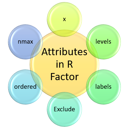
factor(<x>,<levels>,<labels>,<exclude>,<ordered>,<nmax>)

Where x, levels, labels, exclude, ordered, nmax are attributes of factors.

Example: Consider the input vector in our example blood, which we created in our above session. The factor can be created out of input vector blood by using the factor(). Here the syntax uses only attribute X as the input vector.

blood is the input vector that resembles the attribute X.

factor(blood)

This code gives output as shown below

[1] A  B  AB O  AB A  O  B 
Levels: A AB B O

The output contains no double quotes like that of vector blood displayed under the above topic. In the output, you can determine levels corresponding to the different categories of blood groups. The levels are set to default by R with values A AB B O, in case the user does not specify them.

The programmer or user can also set the order of level while creating a factor by passing an argument level. The following are the steps to proceed while specifying level inside factor syntax

1. Create a vector
2. Create a factor out of a vector by mentioning the name of the vector and setting the level which is a vector created by c() with unique values set for the input vector.

Factor(<name of vector> ,level = c())

#set level 
factor(blood,level = c("O","A","AB","B"))

This code gives an output with a predefined level.

[1] A  B  AB O  AB A  O  B 
Levels: O A AB B

The level = c("O", "A", "AB", "B") is a vector created which sets unique values to the input A B AB O AB A O B . Let us compare the output to understand the difference between both without level and with level while creating a factor data structure in R . The level = c("O", "A", "AB", "B") given along the factor() function

Set the level with user-defined values. The default level for the input vector blood is Levels: A AB B O

Whereas once after setting the level it turns out to be  Levels: O A AB B

Now let us see how to label factors. A label is an optional vector provided in the factor() function to label the levels in the vector. A factor with a label specifies a new name for the categories in our example blood which indirectly means labels change the levels name, if levels are changed it affects the names of our input vectors too. This is because levels and associated input vectors are related.

Factor(<name of vector> ,level = c(),label = c())

#set label
factor(blood,level = c("A","B","AB","O"),label =c("BG_A","BG_B","BG_AB","BG_O"))

This code gives an output by renaming the factor elements.

[1] BG_A  BG_B  BG_AB BG_O  BG_AB BG_A  BG_O  BG_B 
Levels: BG_A BG_B BG_AB BG_O

The label argument renames the factor() elements as shown in the below image, A is renamed as BG_A, B is renamed as BG_B, etc.

R does two things when you call a factor function on a character vector. They are

1. It scans through the vector (blood) to see the different categories such as “A”, ”AB”, ”B", AND “O”.
2. It converts the character vector (blood) to a vector with integer values.

These integers correspond to a set of character values to use when the factor is displayed. This can be inspected by revealing the structure. The structure can be revealed using str()  a built-in function provided by R.

str(factor(blood))

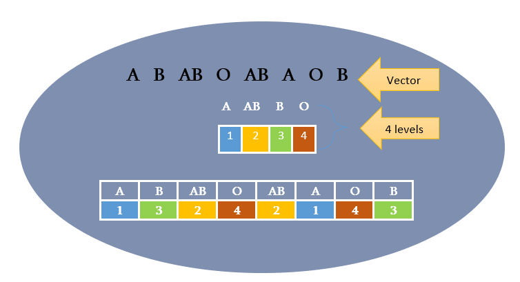
It produces an output that determines the structure of the factor you are dealing with which tells there are 4 levels

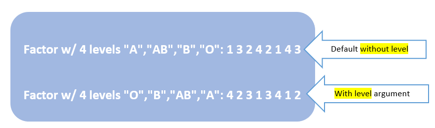
Factor w/ 4 levels "A","AB","B","O": 1 3 2 4 2 1 4 3

The A’s are encoded as 1 because it is the first level. AB is encoded as 2 it is the second level and so on.

Look at the image to get a clear picture.

Why conversion from character to integer is required in the R factor?

Suppose these categorical variables or vectors may contain long characters strings. Each time repeating the character strings per observation can take a lot of memory. By using the conversion from character to an integer it is actually encoding a character with a numerical value like “A” with 1 etc which makes it simple and less memory space utilization.

Thus R automatically infers the factor levels from the vector you pass and order them alphabetically. R also provides the provision to set the order of levels. That is different orders for levels can be specified by passing an argument level inside the factor function.

str(factor(blood, levels = c("O","B","AB","A")))

You can see an argument level inside factor() function specifying the order of blood groups. Here “O” blood groups are set to level 1, ”B” blood groups are set to 2, then “AB” as 3 and “A” as4.

Factor w/ 4 levels "O","B","AB","A": 4 2 3 1 3 4 1 2

When you compare the structures of both, without level and with the level argument in factor() you can find encoding is different now.

Functions in the R factor

In R language there are some built-in functions that allow users to gain information about the factors used in an R program. The below table describes the functionality of different available functions in R.

In the next section of this tutorial, you will learn about each function in detail. Let us begin the discussion with the ordered() function.

Ordered() function in R factors

In R factors are classified as ordered and unordered. By default, R provides order to the factor. In some cases level = c() allows the user to predefine the order of input vectors. We discussed this with an example in the above session under how to create a factor, just refresh the same.

Here the idea is to introduce the ordered() function in A. The ordered() function allows the creation of an ordered factor. The syntax is similar to how we create a factor() function.

ordered(<name of vector> ,level = c())

Consider the input vector X as blood

#create a vector blood using c()
blood <- c("A","B","AB","O","AB","A","O","B")

Use the ordered function syntax to order the input vector blood

#set order
ordered(blood,level = c("O","A","AB","B"))

The resultant output after applying the ordered() function is

[1] A  B  AB O  AB A  O  B 
Levels: O < A < AB < B

How to check if an object is a factor or not in the R programming language?

In R programming language the built-in function is.factor() determines whether the object passed through the function belongs to a factor or not in R. It returns logical values either TRUE or FALSE as a result of is.factor(). You need to pass the name of the object or vector that needs to be determined inside the parentheses ( ) of the function.

is.factor(<object name to check >)

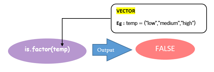
Eg: Given below image checks, temp is a factor or not, passing vector temp as a parameter inside the is.factor().The output is FALSE because the temp is just a vector created using the c() function.

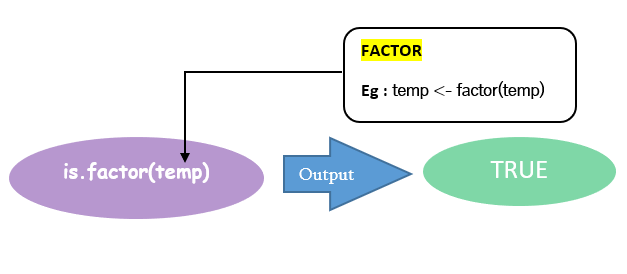
You can make a factor out of this vector(temp) using the factor() function. After that applying is.factor() gives you a logical TRUE as result. Note that the factor created is assigned to a new vector named TEMP.

The steps to identify an object as a factor are

1. Create a vector(object) input
2. Check the vector (object) using is.factor()

Two vectors temp and TEMP are created to observe the differences in each case by comparing their respective outputs.

Let us see how the full source code

#A vector temp is created
temp = c("low","medium","high")
cat("The vector temp is \n :")
print(temp)

#is.factor() checks the object created is a factor or not
cat("Checks the vector temp is a factor \n :")
print(is.factor(temp)  )   #FALSE

#created a factor of temp vector and assigned to vector TEMP
TEMP <- factor(temp)
cat("The factor TEMP is \n :")
print(TEMP)

#is.factor() checks the object created is a factor or not
cat("Checks the factor TEMP is a factor \n :")
print(is.factor(TEMP) )    #TRUE

The output produced is

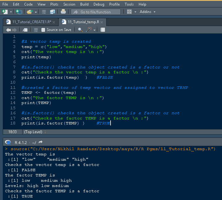
The vector temp is 
 :[1] "low"    "medium" "high"  
Checks the vector temp is a factor 
 :[1] FALSE
The factor TEMP is 
 :[1] low    medium high  
Levels: high low medium
Checks the factor TEMP is a factor 
 :[1] TRUE

The snippet of the same code and output in RStudio is given below

How to convert a variable into a factor in R?

The R programming language supports the conversion of the data type of a variable to a factor or categorical variable. The function as.factor() allows the conversion of character/numeric/integer variables (link to basic data types) of basic data types to the factor data structure.

as.factor(x)

Where x is the input vector or variable.

For example, consider the input vector(X) of a character data type as blood named variable, let us create the variable blood as a vector using the c() function and contains values of character data types.

#create a vector blood using c()
blood <- c("A","B","AB","O","AB","A","O","B")

Let us use as.factor() to convert the vector blood as a factor.

#as.factor()
as.factor(blood)

The output after converting to a factor is

[1] A  B  AB O  AB A  O  B 
Levels: A AB B O

The factor() function as well as as.factor() function are returning a variable of a particular data type as a factor. The performance of as.factor() is greater than factor() function. The is.factor() returns a quick value.

How to check if a factor is ordered or not in R?

The built-in function is.ordered() in R programming language allows one to check whether a defined factor is ordered or not ordered. The logical TRUE or FALSE are returned as output depending upon determining the factor variables. If the variable is a factor returns TRUE else FALSE.

is.ordered(x)

We created in the previous session the blood variable of factor form which we will check here to determine whether it is ordered or not.

#create a vector blood using c()
blood <- c("A","B","AB","O","AB","A","O","B")

#creates a factor
factor(blood)

#is.ordered() 
is.ordered(blood)

The resulting output after execution is

[1] A  B  AB O  AB A  O  B 
Levels: A AB B O

[1] FALSE

The output returns a FALSE which states the factor is not in order. The factor can be ordered either by adding the attribute levels to the function factor() during its creation or by using the function ordered() which seems to be similar to the factor() function but different. Go through the above topics of this tutorial we had discussions regarding the same there with examples.

How to remove the factor element in R?

In R, an argument excludes the element in a factor.

Consider the example TEMP temperature factor created using the factor() function

#created a factor of temp vector and assigned to vector TEMP
TEMP <- factor(temp)
cat("The factor TEMP is \n :")
print(TEMP)

The output generated by factor TEMP is

The factor TEMP is 
 :[1] low medium high  
Levels: high low medium

The above code generated a factor data structure TEMP with factors low, medium, high and by default, their level is specified as high, low, medium.

Now let us include the exclude argument to the factor() function as we did for level, labels. The exclude argument contains the element or factor that needs to be deleted from the TEMP factor. Here in our example medium is getting removed so it is assigned to the argument excluded within double-quotes.

TEMP <- factor(temp,exclude = "medium")

Let us see what happens to the original output after excluding medium from the factor TEMP.

[1] low  <na> high
Levels: high low

In the output, you can see medium is excluded and its position is denoted with <NA> which is a reserved word in R programming language that states not applicable. With the help of excluding the factor levels also get removed.

How to generate factor levels in R?

To generate factor level there is a built-in function gl().The gl() function takes three arguments let it be u,v, labels.

gl(u,v,labels)

Where u is the number of levels get, V is the number of replication, 'labels' is the vector that needs to be passed

Consider the example it contains the number of levels as 3(u), the number of copies or replicas is specified as 2(v) and creates a vector with elements low, high, medium and is passed to argument labels.

gl(3,2,labels = c("low","medium","high"))

The output produced is

[1] low    low    medium medium high   high  
Levels: low medium high

> gl(3,2,labels = c("low","medium","high"))
[1] low    low    medium medium high   high  
Levels: low medium high
> gl(3,2,labels = c("low","medium","high","average"))
[1] low    low    medium medium high   high  
Levels: low medium high average
> gl(4,2,labels = c("low","medium","high","average"))
[1] low     low     medium  medium  high    high    average average
Levels: low medium high average

How do access the components of factors in R?

In R programming language with the help of square brackets [ ] enclosed with the index number of components, you can access any component from a factor. Thus the indexing helps in accessing the components of factors in R.

<name of factor>[<index number of component>]

Consider the people’s blood group example we discussed at the beginning of this tutorial. We will begin by creating vector blood with 8 blood groups as components and by default corresponding levels are also generated.

> blood <- c("A","B","AB","O","AB","A","O","B")
> factor_blood = factor(blood)
> factor_blood 
[1] A  B  AB O  AB A  O  B 
Levels: A AB B O

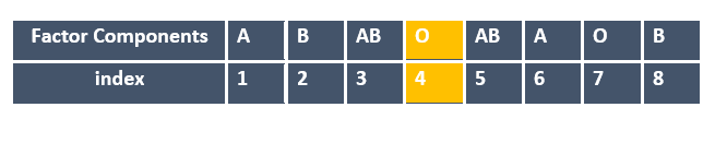
Now let us see how to access the fourth component from the factor named here as factor_blood.

factor_blood[4]

The code returns the element at the fourth (4th) position. Remember index in R starts with 1, not with 0 as in any other language.

[1] O
Levels: A AB B O

The below image shows out of the 8 components A, B, ………, B, the component Oat in the 4th position is retrieved.

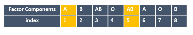
Suppose you want to access more than one component from the factor you created. You can pass the index numbers of components you need to access by building as a vector by creating c().

factor_blood[c(1,5)]

The output is

[1] A  AB
Levels: A AB B O

What happens when you give a negative sign in front of the index number?

factor_blood[-1]

You will get an output as shown below

[1] B  AB O  AB A  O  B 
Levels: A AB B O

All the elements other than the one in the first position are retrieved by specifying -1 in the square bracket.

factor_blood[-5]

The above code removes the 5th component AB from the factor. Compare the output and image we used to show the earlier example.

[1] A  B  AB O  A  O  B 
Levels: A AB B O

How do modify the factor components in R?

The process of modification or changing components in R programming is simple and easy. You need to access the component of the factor as we discussed in our previous topic, after using the syntax to access, mention the new value to be assigned to that particular component.

<name of factor>[index number] = <value to assign>

In the given example

• The name of the factor is factor_blood
• The index number of components is 1
• The value to assign is “AB”

factor_blood[1]="AB"

The code modifies the first component of factor factor_blood, it replaces the original component “A” with the new blood group “AB” assigned to it.